import fdfi
print('FDFI version:', fdfi.__version__)

FDFI version: 0.0.5

OTExplainer: Gaussian Optimal Transport

This tutorial provides a deep dive into the OTExplainer, which uses Gaussian optimal transport for computing feature importance.

What You’ll Learn

1. Mathematical foundation of Gaussian OT

2. Key hyperparameters and their effects

3. When to use OTExplainer vs other methods

4. Best practices for real-world usage

import numpy as np
import matplotlib.pyplot as plt
from fdfi.explainers import OTExplainer

np.random.seed(42)

Mathematical Background

The key insight of OTExplainer is to use the Gaussian optimal transport map to create counterfactual distributions.

Given data \(X\) with mean \(\mu\) and covariance \(\Sigma\), we compute:

\[Z = L^{-1}(X - \mu)\]

where \(\Sigma = LL^T\) (Cholesky decomposition). In Z-space, features are uncorrelated.

To measure the importance of feature \(j\), we:

1. Replace \(Z_j\) with an independent sample from \(N(0, 1)\)

2. Transform back to X-space

3. Compare model outputs

Setup: Create Correlated Data

Let’s create data with correlated features to see how OTExplainer handles dependencies:

# Create covariance matrix with correlations
n_features = 5
correlation = 0.7

cov_matrix = np.eye(n_features)
cov_matrix[0, 1] = cov_matrix[1, 0] = correlation  # Features 0 and 1 are correlated
cov_matrix[2, 3] = cov_matrix[3, 2] = correlation  # Features 2 and 3 are correlated

# Generate correlated data
n_samples = 500
X_train = np.random.multivariate_normal(
    mean=np.zeros(n_features),
    cov=cov_matrix,
    size=n_samples
)

print("Correlation matrix of training data:")
print(np.corrcoef(X_train.T).round(2))

Correlation matrix of training data:
[[ 1.    0.71 -0.03 -0.   -0.05]
 [ 0.71  1.    0.02  0.03 -0.06]
 [-0.03  0.02  1.    0.72 -0.02]
 [-0.    0.03  0.72  1.   -0.  ]
 [-0.05 -0.06 -0.02 -0.    1.  ]]

# Create model: only feature 0 matters
def model(X):
    return X[:, 0] ** 2

# Test data
X_test = np.random.multivariate_normal(
    mean=np.zeros(n_features),
    cov=cov_matrix,
    size=50
)

Effect of nsamples

The nsamples parameter controls Monte Carlo variance. Let’s see its effect:

# Compare different nsamples values
nsamples_values = [10, 50, 200]
results_by_nsamples = {}

for ns in nsamples_values:
    explainer = OTExplainer(model, data=X_train, nsamples=ns)
    results_by_nsamples[ns] = explainer(X_test)

# Plot comparison
fig, axes = plt.subplots(1, len(nsamples_values), figsize=(12, 4))
for ax, ns in zip(axes, nsamples_values):
    phi = results_by_nsamples[ns]["phi_X"]
    se = results_by_nsamples[ns]["se_X"]

    ax.bar(range(n_features), phi, yerr=1.96*se, capsize=3)
    ax.set_xlabel("Feature")
    ax.set_ylabel("Importance")
    ax.set_title(f"nsamples={ns}")
    ax.axhline(y=0, color='gray', linestyle='--', alpha=0.5)

plt.tight_layout()
plt.show()

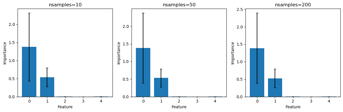
Key observation: Higher nsamples gives smaller error bars (lower variance) but takes longer to compute.

Effect of sampling_method

OTExplainer supports three sampling methods for counterfactual generation:

# Compare sampling methods
sampling_methods = ["resample", "permutation", "normal"]
results_by_method = {}

for method in sampling_methods:
    explainer = OTExplainer(
        model,
        data=X_train,
        nsamples=100,
        sampling_method=method
    )
    results_by_method[method] = explainer(X_test)

# Compare results
print("Feature importance by sampling method:")
print("-" * 50)
print(f"{'Feature':>8}", end="")
for method in sampling_methods:
    print(f"{method:>12}", end="")
print()
print("-" * 50)

for i in range(n_features):
    print(f"{i:>8}", end="")
    for method in sampling_methods:
        phi = results_by_method[method]["phi_X"][i]
        print(f"{phi:>12.4f}", end="")
    print()

Feature importance by sampling method:
--------------------------------------------------
 Feature    resample permutation      normal
--------------------------------------------------
       0      1.3690      1.3081      1.3115
       1      0.5196      0.5108      0.5431
       2      0.0020      0.0020      0.0019
       3      0.0003      0.0003      0.0003
       4      0.0030      0.0029      0.0030

Sampling methods explained:

• resample: Sample from the background data (preserves marginal distribution)

• permutation: Permute values within test set (no new values introduced)

• normal: Sample from standard normal (strongest Gaussian assumption)

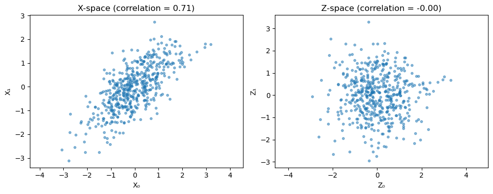
Visualizing the Z-space Transformation

Let’s visualize how OTExplainer transforms correlated data to uncorrelated Z-space:

# Create explainer and access internal matrices
explainer = OTExplainer(model, data=X_train, nsamples=50)

# Transform to Z-space
Z_train = (X_train - explainer.mean) @ explainer.L_inv

# Plot X-space vs Z-space
fig, axes = plt.subplots(1, 2, figsize=(10, 4))

# X-space (correlated)
axes[0].scatter(X_train[:, 0], X_train[:, 1], alpha=0.5, s=10)
axes[0].set_xlabel("X₀")
axes[0].set_ylabel("X₁")
axes[0].set_title(f"X-space (correlation = {np.corrcoef(X_train[:, 0], X_train[:, 1])[0, 1]:.2f})")
axes[0].axis('equal')

# Z-space (uncorrelated)
axes[1].scatter(Z_train[:, 0], Z_train[:, 1], alpha=0.5, s=10)
axes[1].set_xlabel("Z₀")
axes[1].set_ylabel("Z₁")
axes[1].set_title(f"Z-space (correlation = {np.corrcoef(Z_train[:, 0], Z_train[:, 1])[0, 1]:.2f})")
axes[1].axis('equal')

plt.tight_layout()
plt.show()

Shared Diagnostics and Summary

Use the built-in diagnostics and summary() methods for consistent reporting across OT/EOT/Flow explainers.

_ = explainer(X_test)
diag = explainer.diagnostics
print("OT diagnostics")
print("-" * 50)
print(f"Latent independence (median dCor): {diag['latent_independence_median']:.6f} [{diag['latent_independence_label']}]")
print(f"Distribution fidelity (MMD):       {diag['distribution_fidelity_mmd']:.6f} [{diag['distribution_fidelity_label']}]")

print("\nX-space summary")
_ = explainer.summary(alpha=0.05, target='X', alternative='greater')

OT diagnostics
--------------------------------------------------
Latent independence (median dCor): 0.066532 [GOOD]
Distribution fidelity (MMD):       0.000000 [GOOD]

X-space summary
==============================================================================
Feature Importance Results
==============================================================================
Method: OTExplainer
Number of features: 5
Significance level: 0.05
Alternative: greater
Margin method: gap
Practical margin: 0.0031
------------------------------------------------------------------------------
 Feature   Estimate    Std Err   CI Lower   CI Upper    P-value   Sig
------------------------------------------------------------------------------
       0     1.3843     0.5065     0.5511        inf     0.0032   ***
       1     0.5322     0.1313     0.3163        inf     0.0000   ***
       2     0.0020     0.0026    -0.0023        inf     0.6592
       3     0.0003     0.0026    -0.0039        inf     0.8615
       4     0.0031     0.0027    -0.0013        inf     0.5000
==============================================================================
Significant features: 2 / 5
---
Signif. codes:  0 '***' 0.01 '**' 0.05 '*' 0.1 ' ' 1
==============================================================================

Best Practices

When to use OTExplainer

✅ Good for:

• Continuous features

• Roughly Gaussian data

• Fast computation

• Stable results

❌ Consider EOTExplainer for:

• Heavily non-Gaussian data

• Multimodal distributions

• Mixed categorical/continuous features

Recommended settings

explainer = OTExplainer(
    model,
    data=X_train,
    nsamples=50,               # Good balance of speed/accuracy
    sampling_method="resample", # Preserves marginal distribution
)

Summary

Key takeaways:

1. OTExplainer uses Gaussian OT to disentangle correlated features.

2. Higher nsamples reduces variance at the cost of computation time.

3. sampling_method="resample" is recommended for most cases.

4. The transformation to Z-space removes correlations for clean attribution.

5. Shared diagnostics and summary() provide standardized inference reporting.